On the periodic subsampling of linear models in time-series forecasting
Vlad Pyltsov - March 2026
(Read time - 15 min) Linear models have shown surprisingly strong performance in time series forecasting.
This post explores periodic subsampling - a simple technique that groups input data by periodicity
and trains separate linear layers on each group. I provide a conceptual and theoretical rationale,
conduct experiments on mainstream benchmarked datasets, and discuss the implications.
In this blog post, I consider one of the, to my mind, a bit overlooked subfields in time-series forecasting.
In particular, I consider the lightweight models, under which linear models fall pretty naturally.
Historically, initial efforts in the field were focused on complex architectures and looked to show that Deep Learning models, with some tweaks, can be applied to time-series forecasting, for example Informer (Zhou et al., 2021) and Autoformer (Wu et al., 2021).
Notably those two papers compare their models to baselines like LSTMs, which you do not see in the more recent literature.
One of the first papers to essentially break the trend and show that lightweight models can achieve competitive performance is the work by Zeng et al. (2022), where the authors propose a simple linear model with a single fully-connected layer.
The models proposed were described by the authors as "embarrassingly simple".
This essentially opened a new line of research, where the focus shifted to considering lightweight architectures and showing that they can achieve competitive performance with the more complex models.
Certain aspects, like parameter count and training time, became highlighted factors in the overall evaluation.
While the modern literature is rich in the variety of proposed lightweight models, I will outline a few works, which I find particularly interesting.
To begin with, I want to highlight Toner et al. (2024) work, in which they provide a rigorous analysis on the linear models.
In partuclar, they show that from theoretical perspective different linear models are essentially identical (i.e., any affine linear map is mutually expressible).
From practical perspective, they show that a simple OLS outperforms the Linear models on most of the mainstream datasets.
Next, the work by Xu et al. (2023) proposes a model, which transforms data into frequency domain before passing it to linear layer.
They also introduce a low-pass filter, which preserves frequency components only above a cut-off threshold, and, notably, the model only operates on 10-k parameters.
Lastly, I also want to highlight the work by Lin et al. (2024).
In this work, the authors propose to remove the recurring cyclical components before passing through the linear layer and then add them back to the output.
The removal of the recurrent cycles is also modeled and is learnable.
Other notable works of the more recent literature include but are not limited by the works by Si et al. (2025), Yue et al. (2025), and Yue et al. (2025).
Among the works mentioned above, one of the works particularly stands out to me, which is the model by Lin et al. (2024).
In this work, the authors come up with an architecture, which is able to represent time-series data with only 1-k parameters.
They call it SparseTSF. So, how were they able to achieve such a low parameter count?
In fact, not only achieve a low parameter count, but also achieve competitive performance with the more complex models?
The key to this is the periodic subsampling of the input data.
The authors essentially propose to subsample the input data with a certain period, which is a hyperparameter of the model, and then pass the subsampled data through a linear layer.
The output of the linear layer is then upsampled back to the original length and added to the input data.
What is this periodic subsampling? Imagine you have a time-series data with a certain length, say 720 - a typical lookback length in the litersture.
Now, if you subsample this data with a period of 24, you will essentially be taking every 24-th data point, which will give you a subsampled data of length 30.
In their work, they mostly use a period of 24, which is a natural choice for time-series data with daily cycles (i.e., taking points every hour).
Now, the way the sampled vectors are passed to linear layer is also interesting.
Back to our example, if we have subsampled data of 24 periods for 720 data points, we will have 24 vectors of length 30.
The input dimension in this case becomes the length of the vectors, which is 30.
The output dimension is a similar length, but the horizon divided by the period, which, for example if the horizon is 720, would also be 720/24 = 30.
Hence, the linear layer, which serves as a backbone of the most parameter count, in this case will have 30*30 = 900 parameters.
In this sense, having the 900 parameters in the linear layer is much less than a typical linear layer which is 720*720 = 518,400 parameters.
The authors also propose using a convolutional layer before sampling in order to preserve some local context.
This idea has some pretty strong parallel to the idea to use hourly disaggregated models for regressive load forecasting (Hu et al., 2023).
The main difference is that instead of lookback window, the input for the regressive setting are exogenous variables.
Since the performance of the idea is strong, I got curious about the potential of using the periodic subsampling strategy exclusively with the linear models, without the convolutional layer, and also applying separate linear layers for each of the sampled vectors, which is a bit different from the SparseTSF architecture.
In further sections, I will provide some theoretical rationale for the potential of the periodic subsampling strategy and then provide some experimental results on mainstream datasets.
Theory and Motivation
Now, before going into the experiments, I want to provide some theoretical rationale for the potential of the periodic subsampling strategy.
One of the interesting aspects of the linear models is that it turned out that they are not very good in capturing trend.
This observation was made in the work by Li et al. (2023), where they showed how Reverse Instance Normalization (RevIN) can scale each segment into the same range for the trend signal.
This can be thought, to a certain degree, of allowing the linear layer to focus on learning the periodic components, which are more easily learnable by the linear layer, by turning some trends into seasonality.
On one hand, the periodic subsampling strategy can be seen as a way to further facilitate the learning of the periodic components by essentially forcing the model to focus on the periodicity of the data.
On the other hand, the periodic subsampling is exactly the decomposition of the time-series into periodic trends itself if the data are perfectly periodic.
To illustate the idea, consider the time series of seasonal and trend components:
\[x(t) = s(t) + p(t)\]
where \(s(t)\) is the seasonal component and \(p(t)\) is the periodic component.
Suppose the seasonal component has a period of \(w\), which means that \(s(t) = s(t + w)\) for all \(t\).
We can establish the following theorem:
>
Theorem: If the time series \(x(t)\) is perfectly periodic with period \(w\), then the periodic subsampling of \(x(t)\) with period \(w\) results in a set of binned time series, each of which has a constant seasonal component and a resampled trend component.
More formally, for each bin \(b\) (i.e., the periodically sampled vector), the binned time series \(x^{b}(t) = x(kw + b) = s(kw + b) + p(kw + b)\), has the form
\(x^{b}(t) = c_b + p^{b}(t)\), where \(c_b = s(b)\) is a constant (i.e., the value of the seasonal component at phase \(b\)) and \(p^{b}(t)= p(kw + b)\) is a resampled version of the trend component.
Now, consider a more complicated time series, which has the form of:
\[x(t) = s(t)p_1(t) + p_2(t)\]
where \(s(t)\) is the seasonal component, \(p_1(t)\) is a periodic trend component, and \(p_2(t)\) is a non-periodic trend component.
We can establish the following theorem:
>
Theorem: If the time series \(x(t)\) is of the form \(x(t) = s(t)p_1(t) + p_2(t)\), where \(s(t)\) is a periodic seasonal component, \(p_1(t)\) is a periodic trend component, and \(p_2(t)\) is a non-periodic trend component, then the periodic subsampling strategy can be used to isolate and model each component separately.
More formally, for each bin \(b\), the binned time series has the form \(x^{b}(t) = c_b \cdot p_1^{b}(t) + p_2^{b}(t)\), where \(c_b = s(b)\) is a constant, \(p_1^{b}(t)= p_1(kw + b)\) and \(p_2^{b}(t)= p_2(kw + b)\) are resampled versions of the trend components.
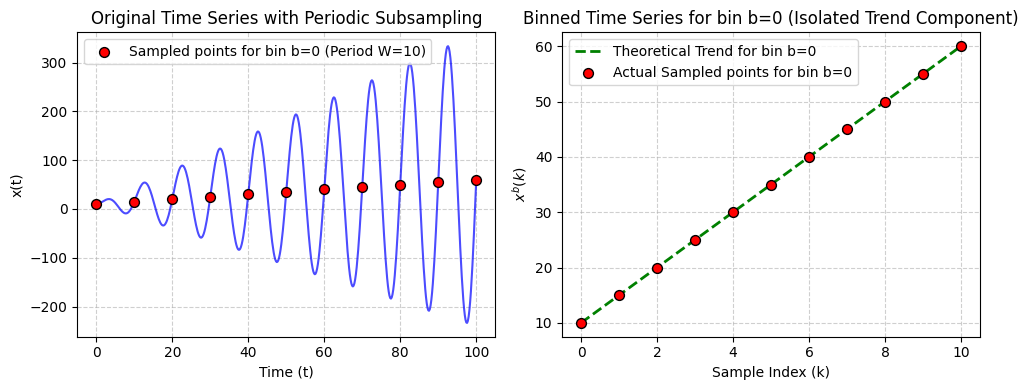
The concept can be seen on the plot below:
Figure 1: Theoretical Illustration of the periodic subsampling strategy.
Essentially, with pretty stochastic data on the left, subsampling allows us to pass a clean trend component to the linear layer.
Since RevIN allows the linear model to process the trend component more effectively, the combination of the periodic subsampling and RevIN can be particularly interesting for time-series data with strong periodicity and trends.
Whether the data actually exhibit such properties and whether subsampling actually can provide theoretical benefits is an empirical question, which I will try to answer in the next section.
Experiments
I conduct experiments on the mainstream datasets, such as ETTh1, and compare the performance of the linear model with and without the periodic subsampling strategy.
For the sampled model, I use individual linear layers for each of the sampled vectors, which is a bit different from the SparseTSF architecture, where the same linear layer is used for all the sampled vectors.
Additionally, I also experiment with the combination of the periodic subsampling strategy and RevIN. In particular, for the subsampled model, I apply RevIN to each of the sampled vectors separately before passing them through the linear layers or globally to the entire input vector.
Lastly, I also iterate a modified version of SparseTSF without the convolutional layer. The results are provided in the table below.
Table 1: Comparison of results between models. The top three results are highlighted in bold. The look-back length \(L\) for all models is uniformly set to 720, and the forecast horizon \(H\) in \( \{96, 192, 336, 720\} \). For ETTh1, ETTh2, and Electricity the periodicity was set to 24, and for ETTm1 and ETTm2 to 4.
Models
Linear
RLinear
BinnedLinear
BinnedGlobal RLinear
BinnedEach RLinear
SparseTSF (no conv)
Dataset
H
MSE
MAE
MSE
MAE
MSE
MAE
MSE
MAE
MSE
MAE
MSE
MAE
ETTh1
96
0.390
0.414
0.388
0.410
0.397
0.406
0.371
0.389
0.372
0.389
0.371
0.388
192
0.413
0.423
0.420
0.428
0.431
0.429
0.417
0.415
0.417
0.413
0.415
0.412
336
0.467
0.467
0.451
0.447
0.464
0.455
0.452
0.434
0.453
0.429
0.448
0.429
720
0.501
0.512
0.474
0.479
0.504
0.514
0.469
0.473
0.480
0.457
0.432
0.446
ETTh2
96
0.297
0.363
0.275
0.340
0.339
0.395
0.292
0.351
0.292
0.351
0.296
0.349
192
0.390
0.424
0.332
0.380
0.433
0.453
0.346
0.390
0.344
0.388
0.345
0.381
336
0.507
0.494
0.366
0.410
0.533
0.513
0.367
0.412
0.368
0.412
0.360
0.399
720
0.851
0.659
0.413
0.447
0.832
0.652
0.414
0.448
0.422
0.452
0.384
0.425
ETTm1
96
0.309
0.353
0.327
0.367
0.318
0.363
0.315
0.357
0.317
0.357
0.322
0.362
192
0.339
0.371
0.352
0.381
0.344
0.376
0.345
0.374
0.343
0.372
0.340
0.370
336
0.385
0.411
0.380
0.397
0.383
0.405
0.374
0.391
0.370
0.387
0.382
0.400
720
0.423
0.424
0.429
0.424
0.433
0.436
0.418
0.413
0.417
0.412
0.425
0.419
ETTm2
96
0.166
0.261
0.172
0.266
0.166
0.259
0.166
0.256
0.167
0.259
0.167
0.257
192
0.227
0.307
0.225
0.301
0.225
0.307
0.219
0.294
0.219
0.294
0.220
0.294
336
0.294
0.356
0.280
0.338
0.277
0.338
0.273
0.331
0.271
0.330
0.276
0.332
720
0.387
0.417
0.362
0.391
0.407
0.426
0.363
0.390
0.354
0.387
0.350
0.379
Electricity
96
0.141
0.243
0.133
0.228
0.140
0.235
0.140
0.234
0.140
0.233
0.140
0.233
192
0.154
0.254
0.164
0.265
0.153
0.248
0.153
0.245
0.153
0.244
0.152
0.245
336
0.169
0.271
0.180
0.280
0.167
0.263
0.168
0.261
0.169
0.260
0.168
0.261
720
0.205
0.306
0.204
0.292
0.204
0.297
0.206
0.293
0.208
0.293
0.206
0.294
Firstly, one of the observations is that the sampled models perform better except on the ETTh2 dataset.
This observation is pretty striking meaning that looking at the periodic components separately without mixing them can be more effective than looking at the whole sequence at once.
Secondly, SparseTSF, even without the convolutional layer, performs better than denser linear models, especially on the ETTh datasets.
This suggests that subsampling does not even need an additional parameter overhead to be effective.
Neverthless, the convolutional layer does provide a boost in performance on the ETT datasets (results can be found in their paper), which suggests that losing the local context in the subsampling process is not always optimal.
Lastly, the difference between global and separate RevIN strategies is rather marginal.
This potentially suggests that distributioal shifts in the subsampled sequences are similar to those in the original sequence, and thus, the same normalization strategy does not yield improvements.
Discussion
One caveat is the ETTh2 dataset, where periodic subsampling hurts performance across all models.
To understand why, a simple variance decomposition can be performed.
The idea is to measure how much of the total variance in each lookback window is explained by the sample-specific means - that is, the periodic component that subsampling isolates.
Concretely, for each lookback window, the sample means are computed (i.e., the average value within each periodic sample), and the variance of these sample means is compared to the total variance of the sequence.
A high ratio indicates strong periodic structure that subsampling can exploit; a low ratio means most of the variation comes from trend or noise, which gets fragmented across samples.
The formula for it looks like this:
\[\text{Periodic Var \%} = \frac{1}{CN} \sum_{c=1}^{C} \sum_{n=1}^{N} \frac{\text{Var}(\hat{x}^{(c,n)}_{t_n:t_n+L-1})}{\text{Var}(x^{(c,n)}_{t_n:t_n+L-1})} \times 100\%\]
where \(C\) is the number of channels, \(N\) is the number of samples, \(\hat{x}^{(c,n)}\) is the sequence of sample means for channel \(c\) and sample \(n\), and \(x^{(c,n)}\) is the original sequence.
This analysis reveals that only about 14% of ETTh2's variance originates from sample-specific means, compared to over 56% for ETTh1 and 82% for Electricity.
When the periodic signal is this weak, subsampling forces separate models to learn from a structure that explains very little of the data, while the remaining variation gets split across samples without meaningful decomposition.
This suggests a practical implication: periodic subsampling is most effective when the data exhibits strong periodic characteristics, and can be counterproductive otherwise.
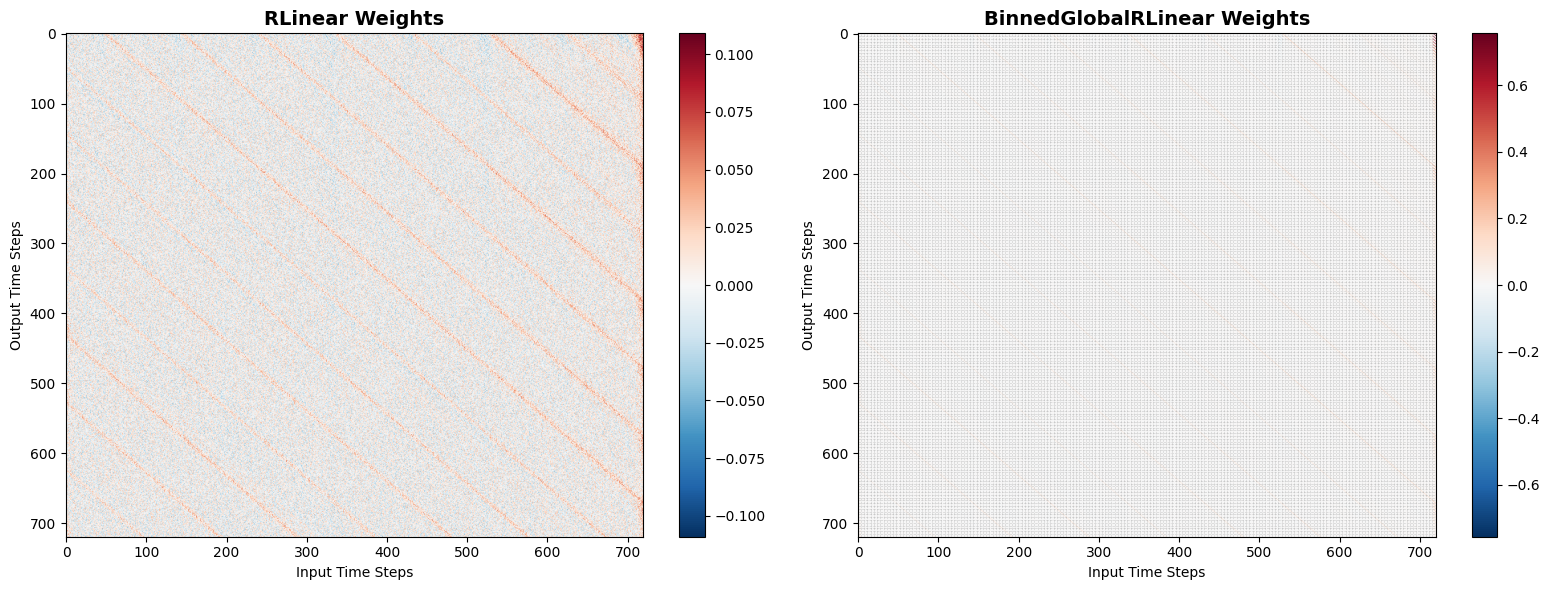
One interpretation is to see how the sampling strategy acts on weights of the models. Consider two plots below.
Figure 2: Weight Illustration of the periodic subsampling strategy (ETTm1 dataset).
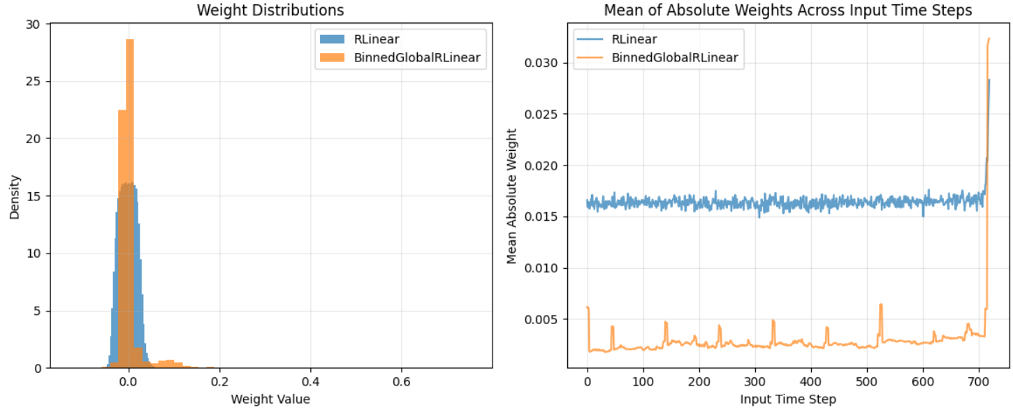
Figure 3: Weight Distribution Illustration of the periodic subsampling strategy (ETTm1 dataset).
It can be seen that the sampled model has a more structured weight pattern, with certain weights being more prominent than others, which suggests that the model is learning to focus on specific periodic components.
The mean absolute weights also have periodic spikes that align with the sampling period.
For the fully-connected model, the weights are more uniformly distributed and concentrate around 0, spreading its reliance more evenly across all features.
The sampled model's weight distribution is more skewed, with a noticable small tail, indicating that it relies more heavily on certain features corresponding to the periodic samples.
Conclusion
In summary, the periodic subsampling strategy can be a powerful tool for time series forecasting when the data has strong periodic components.
It allows models to focus on these components separately, which can lead to improved performance and reduced parameter counts.
From practical persepctive, the implication is the assessment of the periodic structure before applying this strategy, as it can be detrimental when the periodic signal is weak.
Future work could explore adaptive subsampling strategies that dynamically adjust the sampling period based on the data's characteristics, or hybrid models that combine subsampled and full-sequence processing to capture both periodic and non-periodic patterns effectively.
Moreover, investigating the theoretical underpinnings of why subsampling works in certain contexts and not others could provide deeper insights into the nature of time series data and model architectures.
If you found this interesting or have any questions, please feel free to reach out to me via email.